The German tank problem
2024-02-24
Probability StatisticsContents
- 1 Introduction
- 1.1 Abbreviations and symbols used throughout this post
- 2 Assumptions
- 3 Frequentist approach
- 3.1 Maximum likelihood estimator
- 3.2 Suppose we fixed the maximum observed serial number m. How does the likelihood function behave with sample size k?
- 3.3 Minimum variance unbiased estimator
- 3.4 Derivation of an unbiased estimator
- 3.5 Showing this is in fact the minimum variance unbiased estimator
- 4 Bayesian approach
- 4.1 Comparison between frequentist and Bayesian approaches
- 4.2 Exploring the Bayesian posterior PMF
- 4.3 Suppose we 'get lucky' on the first sample and it happens to contain the highest serial number. How does the posterior behave in this case as we collect more data?
- 4.4 Suppose the highest serial number observed in a sample is equal to the sample size. How does the posterior behave in this case as a function of sample size?
- 5 Conclusion
- 6 References
1 Introduction
During WW2, the Allies faced the problem of estimating the monthly rate of German tank production from very limited data. Under a set of assumptions which were justified at the time, it was possible for them to achieve this accurately using statistical methods. In this article, I will outline some of these methods.
The phrase German tank problem has come to refer to the general problem of estimating the maximum of a discrete uniform distribution from sampling without replacement.
1.1 Abbreviations and symbols used throughout this post
The following is a list of abbreviations I use throughout this post:
| Abbreviation | Meaning |
|---|---|
| GTP | German tank problem |
| LF | Likelihood function |
| MAP | Maximum a posteriori estimator |
| MLE | Maximum likelihood estimator |
| MVUE | Minimum variance unbiased estimator |
| PMF | Probability mass function |
The following is a list of symbols I use throughout this post:
 is a random sample of tanks
 is the size of this sample
 is the maximum serial number observed in this sample
 is the total number of tanks
2 Assumptions
Let's make the following assumptions:
- The serial numbers indeed count the number of tanks. E.g. the 1st tank manufactured had serial number 1 (or probably something resembling #00001), the 2nd had serial number 2, the
 th had serial number .
 - The probability of observing a given serial number from the total population of tanks having total number follows a discrete uniform distribution, i.e.
 .
.
With these assumptions in place, let's proceed with our analysis.
There are 2 key approaches we can take, corresponding to the 2 popular interpretations of probability theory:
- Frequentist
- Bayesian
3 Frequentist approach
In the frequentist approach, we:
- Ask for a single point estimate of ; and
- Ask how confident we are in our estimate.
To answer Question 1, we need an estimator for ![]() . We will consider 2 estimators: The maximum likelihood estimator (MLE) and the minimum variance unbiased estimator (MVUE).
. We will consider 2 estimators: The maximum likelihood estimator (MLE) and the minimum variance unbiased estimator (MVUE).
To answer Question 2, we calculate confidence intervals for our selected estimator. For sake of brevity, I will not discuss this in this post.
3.1 Maximum likelihood estimator
In frequentist analysis, a popular estimator is the maximum likelihood estimator, which is the maximum of the likelihood function. The likelihood function looks identical to the joint probability density of the observed data, except that we consider it not as function of the data (like the joint PMF is), but as a function of the parameters PMF. It is a term that appears in Bayes' theorem.
What is our data, and what are the parameters of our density? Our data are the observed serial numbers. The single parameter - the one we wish to estimate - is the upper bound of the uniform PMF we have assumed in Assumption 2.
To derive the likelihood function, first consider the case where we have observed the serial number of only a single tank. In this case, under Assumption 2, the joint density (in this case, just the 'density') is simply the univariate discrete uniform PMF with bounds ![]() :
:
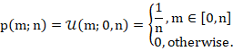
This PMF is familiar, and for ![]() looks like:
looks like:
This of course is a function of ![]() . Now, to go from this to the likelihood function, instead of fixing the parameter
. Now, to go from this to the likelihood function, instead of fixing the parameter ![]() and considering it a function of
and considering it a function of ![]() , we fix an
, we fix an ![]() and consider it as a function of
and consider it as a function of ![]() . We write
. We write ![]() to refer to the likelihood.
to refer to the likelihood.
For example, suppose we have observed ![]() . This sole data point is our dataset. The likelihood function looks like this:
. This sole data point is our dataset. The likelihood function looks like this:
Note that, because that the LF is a function of the parameter ![]() and not a function of the data
and not a function of the data ![]() , the LF is not a PMF and thus is not normalised.
, the LF is not a PMF and thus is not normalised.
Now, consider the case where we have observed the serial numbers of 2 tanks. If, hypothetically, we were sampling with replacement (capturing a tank, recording the serial number, and then returning it to the enemy!), the samples would be independent and the joint density would be simply the bivariate discrete uniform PMF with bounds ![]() .
.
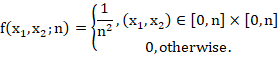
But this, of course, is NOT what we're doing. We are sampling without replacement. So the samples are NOT independent. The density is thus:
In the general case of ![]() tanks, the density is:
tanks, the density is:
Where ![]() .
.
To get the likelihood function from this, you simply consider it as a function of ![]() instead of X. We write:
instead of X. We write:
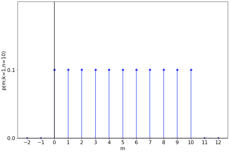
For example, suppose ![]() . The following figure displays the likelihood function in this case.
. The following figure displays the likelihood function in this case.
3.2 Suppose we fixed the maximum observed serial number m. How does the likelihood function behave with sample size k?
Let's normalise the two likelihood functions and superimpose them:
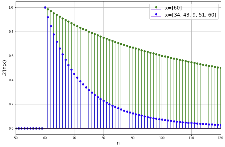
Compared to the case of a single observation (![]() ), the LF decays more rapidly when
), the LF decays more rapidly when ![]() . Intuitively, this is because the larger your sample size, the more confident you are that its maximum is the true maximum.
. Intuitively, this is because the larger your sample size, the more confident you are that its maximum is the true maximum.
Finally, the MLE is simply the value that maximises the LF. Having derived the likelihood function, we can immediately see that the MLE is simply the sample maximum, in this case 60.
3.3 Minimum variance unbiased estimator
Now, there's a problem with the MLE in this case: It is biased, which means that its expected value is not equal to the true value. In fact, 'most of the time', the MLE will underpredict the true value, 'sometimes' it will get it right, but it can NEVER overpredict it. It is 'biased downward'.
So instead, we look for an unbiased estimator.
3.4 Derivation of an unbiased estimator
An unbiased estimator ![]() for
for ![]() , is one whose expected value is equal to
, is one whose expected value is equal to ![]() .
.
To derive this, first, let's consider the expected value of the sample maximum, ![]() . It is possible to show that:
. It is possible to show that:
See, for example, Example 5.1.2 of Hogg et. al. (2019). Rearranging this,
![]()
Now, from the linearity of the expectation operator, we can bring the factor ![]() and the
and the ![]() inside the expectation operator:
inside the expectation operator:
![]()
Thus, we have found something whose expected value is equal to ![]() . Thus, the estimator
. Thus, the estimator
![]()
Is an unbiased estimator for ![]() .
.
3.5 Showing this is in fact the minimum variance unbiased estimator
As it turns out, this estimator is in fact the minimum variance unbiased estimator (MVUE) of ![]() . The proof is beyond the scope of this post, but essentially what you need to do is:
. The proof is beyond the scope of this post, but essentially what you need to do is:
- Show that the sample maximum is a sufficient statistic for the population maximum.
- Show that it is also a complete statistic for the population maximum.
- Invoke the Lehmann-Scheffe theorem, which states that any estimator that is unbiased and depends on the data only through a complete, sufficient statistic is the unique MVUE.
The details are left to the reader.
In this example, the MVUE for ![]() is
is ![]() tanks.
tanks.
In summary, for the frequentist approach, we have:
| Estimator | Value |
|---|---|
| MLE | 60 |
| MVUE | 71 |
4 Bayesian approach
In the Bayesian approach, instead of being interested in a single point estimate of ![]() , we ask for a probability density of n given our assumptions and data. Specifically, we ask for the posterior PMF of
, we ask for a probability density of n given our assumptions and data. Specifically, we ask for the posterior PMF of ![]() having prior observed
having prior observed ![]() and
and ![]() , i.e.
, i.e. ![]() . We can then use various descriptive statistics from the PMF as our estimators. In particular, the mode of the posterior PMF is called the maximum a posteriori (MAP) estimator.
. We can then use various descriptive statistics from the PMF as our estimators. In particular, the mode of the posterior PMF is called the maximum a posteriori (MAP) estimator.
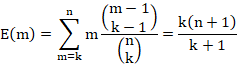
The posterior PMF can be expressed using Bayes' rule as:
I have decided to omit the details from this post, but in summary, each of these are:
Substituting these into Bayes' rule,
![]()
Example
Suppose we observe ![]() , as before. The posterior PMF in this case is shown in the following figure.
, as before. The posterior PMF in this case is shown in the following figure.
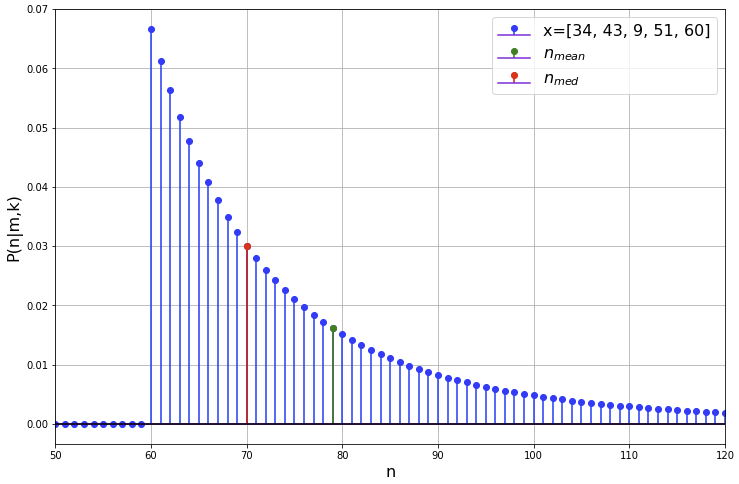
The posterior mode (MAP), median and mean are shown in the following table.
| Estimator | Value |
|---|---|
| Posterior mode (MAP) | 60 |
| Posterior mean | 79 |
| Posterior median | 70 |
4.1 Comparison between frequentist and Bayesian approaches
In summary, we have:
| Approach | Estimator | Value |
|---|---|---|
| Frequentist | MLE | 60 |
| Frequentist | MVUE | 71 |
| Bayesian | Posterior mode (MAP) | 60 |
| Bayesian | Posterior mean | 79 |
| Bayesian | Posterior median | 70 |
Observations:
- We know the frequentist MLE is biased and will tend to underestimate the true value of .
- The frequentist MVUE provides an unbiased estimate of in the sense that its expected value is equal to .
- When we look at the Bayesian results, the posterior PMF has positive skewness, so the posterior mean may not be the most meaningful estimate.
- The posterior median is in close agreement with the frequentist MVUE.
4.2 Exploring the Bayesian posterior PMF
In this last section, I will ask and answer some basic questions to provide some intuition behind the Bayesian approach.
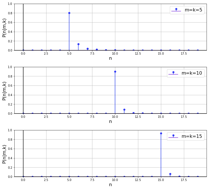
4.3 Suppose we 'get lucky' on the first sample and it happens to contain the highest serial number. How does the posterior behave in this case as we collect more data?
The results of a quick simulation of this case are shown below. What we can say is that, given fixed ![]() , with increasing
, with increasing ![]() , the probability mass at
, the probability mass at ![]() increases. As in the case of the likelihood function in the frequentist case from before, this is intuitive, since a larger sample size gives you more confidence that the observed maximum serial number is the total number of tanks. In the limit
increases. As in the case of the likelihood function in the frequentist case from before, this is intuitive, since a larger sample size gives you more confidence that the observed maximum serial number is the total number of tanks. In the limit ![]() , the PMF becomes a single spike of probability mass 1.0 at
, the PMF becomes a single spike of probability mass 1.0 at ![]() .
.
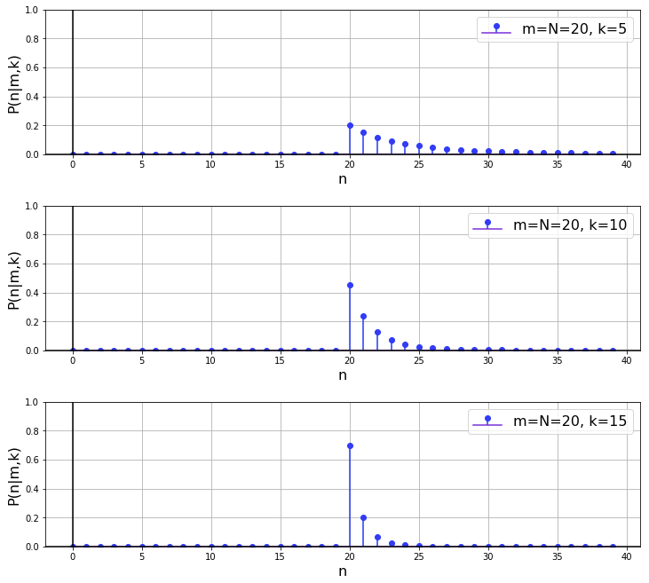
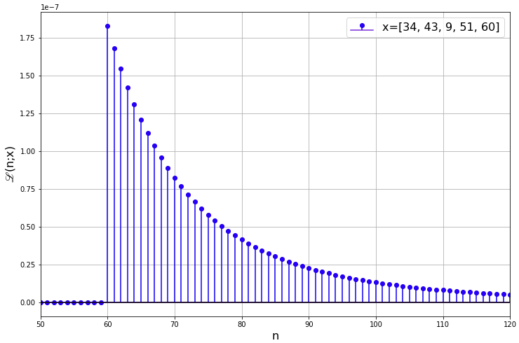
4.4 Suppose the highest serial number observed in a sample is equal to the sample size. How does the posterior behave in this case as a function of sample size?
The results of a quick simulation of this case are shown below. What we can say is that, setting ![]() , the credibility that
, the credibility that ![]() increases with increasing
increases with increasing ![]() , as shown by the fact that there is more mass at
, as shown by the fact that there is more mass at ![]() (the PMF isn't merely shifted to the right). This is because, from Bayes' rule, the posterior PMF is proportional to the LF, which, as we've seen in the frequentist approach, becomes 'steeper' with increasing sample size.
(the PMF isn't merely shifted to the right). This is because, from Bayes' rule, the posterior PMF is proportional to the LF, which, as we've seen in the frequentist approach, becomes 'steeper' with increasing sample size.
We can interpret this intuitively as follows: Suppose we don't know ![]() and we draw the sample
and we draw the sample ![]() . While this is compelling evidence that
. While this is compelling evidence that ![]() , it isn't as compelling as the evidence that, say,
, it isn't as compelling as the evidence that, say, ![]() if the sample we draw is
if the sample we draw is ![]() .
.
5 Conclusion
In this post, we have explored two approaches to the German tank problem - the problem estimating the maximum of a discrete uniform distribution from sampling without replacement. We have explored frequentist and Bayesian approaches and compared their results.
6 References
https://en.wikipedia.org/wiki/Lehmann%E2%80%93Scheff%C3%A9_theorem