Derivation of Glorot initialisation
2024-03-08
Machine learning Deep learning Neural networksContents
- 1 Introduction
- 2 Intended audience
- 3 What is Glorot initialisation?
- 4 Brief outline of Glorot et al's derivation
- 5 My commentary on Glorot et al's derivation
- 5.1 Prelude: Desirable statistical properties of the activation vectors and cost function gradients of a neural net at initialisation
- 5.2 Assumptions used in the derivation
- 5.3 Note: Formatting for Glorot et al's work vs. my commentary
- 5.4 Start of the derivation
- 6 Conclusion
- 7 References
1 Introduction
Glorot initialisation (AKA Xavier initialisation) is today the most popular method for initialising the weights of deep neural networks. It was introduced by Xavier Glorot and Yoshua Bengio in a landmark paper [1] published in 2010. Since then, Glorot initialisation has become the default initialisation method in popular deep learning libraries such as Keras/TensorFlow.
In this post, I will derive Glorot initialisation from first principles via a commentary on Glorot et al's paper, referring to his original derivation verbatim and filling in any details where more explanation could be provided for clarity. By keeping consistent with his notation, my intention is that this post can be read directly alongside his paper.
2 Intended audience
The intended audience is those who have some familiarity with neural networks, including units, layers, activation functions, backpropagation etc. who are comfortable reading quantitative arguments expressed using symbols - that is, those who are comfortable reading mathematics.
3 What is Glorot initialisation?
Glorot initialisation is a method for initialising the weights of a neural network in preparation for network training.
In short, Glorot initialisation keeps the variance of the unit activations and cost function gradients approximately the same across all layers at initialisation. It does so by adjusting the variance of the sampling distribution for the weights according to the number of units in their adjacent layers. Specifically, the sampling distribution used for the weights is:

Where ![]() is the weight matrix between layers
is the weight matrix between layers ![]() and
and ![]() ,
, ![]() refers to a uniform distribution and
refers to a uniform distribution and ![]() and
and ![]() are the number of units between layers
are the number of units between layers ![]() and
and ![]() . Thus, the sampling variance decreases with the total number of units in the layers corresponding to the given weight matrix. This is the expression Glorot et. al. derived and will form the subject of this post.
. Thus, the sampling variance decreases with the total number of units in the layers corresponding to the given weight matrix. This is the expression Glorot et. al. derived and will form the subject of this post.
The following is a quick Keras experiment illustrating the idea. To produce the 1st figure, I generated 100 FNNs at random with the same 3-64-32-16-1 architecture (i.e. a model with 3 input features, 3 hidden layers and 1 output), tanh activation functions and Glorot initialisation, performed a single feedforward pass using a dummy input drawn from a trivariate standard normal (0 mean, identity covariance) distribution, and plotted histograms of the resultant activations for the 3 hidden layers. The 2nd figure was produced in the same way except with weights sampled in a 'naive' fashion from a uniform distribution ![]() .
.
As the figures below show, for Glorot initialisation, the variance of the activations remains approximately constant across layers, whereas for naive uniform initialisation, they are different (in fact, orders of magnitude different). Glorot et al showed that, for good training performance, you want the 1st behaviour.
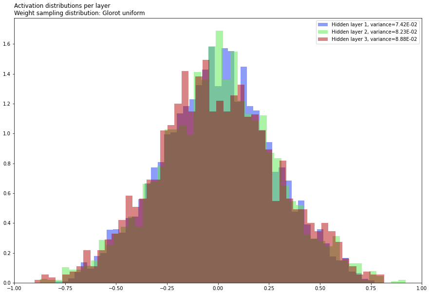
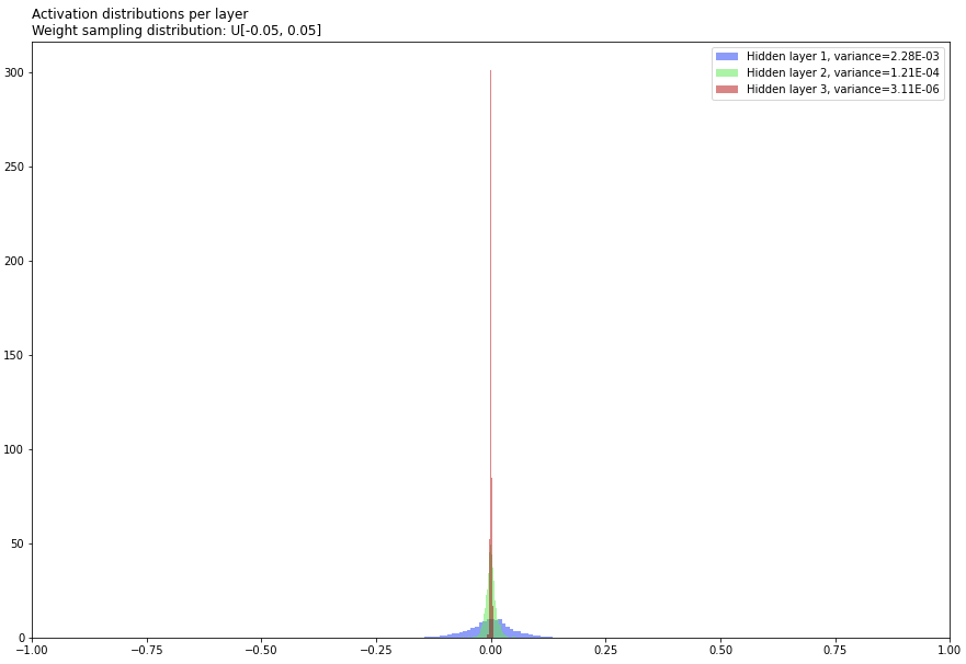
Over a decade since the publishing of their paper, it is now common knowledge that, in general, neural network training performance can be highly sensitive to the method used to initialise the weights.
4 Brief outline of Glorot et al's derivation
A brief outline of Glorot et al's derivation of their initialisation method goes as follows:
- State some desirable statistical properties you would like the activation vectors and cost function gradients to have - specifically, in terms of their variances.
- Derive expressions for these variances in terms of the variance of the weights at each layer.
- Use (1) and (2) to solve for an expression for the desired variance of the weights at each layer.
The derivation can be found on pp. 7 of Glorot et al (2010).
5 My commentary on Glorot et al's derivation
5.1 Prelude: Desirable statistical properties of the activation vectors and cost function gradients of a neural net at initialisation
From the start of the 2nd column in pp. 7:
From a forward propagation POV, to keep information flowing, we would like that
![]()
(8)
In words: We would like the variance of the activations to remain constant across layers.
From a backprop POV, we would similarly like to have
![]()
(9)
In words: We would like the variance of the cost function gradients WRT the pre-activations (sometimes referred to as the 'errors' or 'deltas' ![]() ) to remain constant across layers.
) to remain constant across layers.
I will refer to Eqns. (8) and (9) as the activation variance criterion (AVC) and error variance criterion (EVC), respectively.
5.2 Assumptions used in the derivation
In the following derivation, we make the following assumptions:
- The network we are referring to is a fully connected network, i.e. there is no dropout, weight sharing etc. In other words, it is a vanilla feedforward neural net (FNN).
- The weights in a given layer have a common variance at initialisation.
- The activations in a given layer have a common variance at initialisation.
- The weight distributions for all layers are have expectation zero, i.e.
 .
. - The activation distributions for all layers have expectation zero, i.e.
 .
. - The weights and activations are independent.
5.3 Note: Formatting for Glorot et al's work vs. my commentary
In the following, text in italics is taken verbatim from Glorot et al's paper - it was NOT written by me and I do not claim any credit for it. Text in normal formatting is commentary written by me.
5.4 Start of the derivation
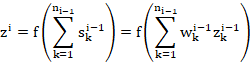
Starting from the 1st paragraph in the 1st column of pp. 7:
For a dense artificial NN using symmetric activation function ![]() with unit derivative at 0 (i.e.
with unit derivative at 0 (i.e. ![]() ), if we write
), if we write ![]() for the activation vector of layer
for the activation vector of layer ![]() , and
, and ![]() the argument vector of the activation function at layer
the argument vector of the activation function at layer ![]() , we have
, we have ![]() and
and ![]() .
.
A quick note: Glorot (2010) calls ![]() the 'argument vector of the activation function at layer
the 'argument vector of the activation function at layer ![]() '. Instead, throughout this post I will use the term 'pre-activation vector of layer
'. Instead, throughout this post I will use the term 'pre-activation vector of layer ![]() '.
'.
As straightforward as this 1st paragraph might be to some, it is worthwhile making a remark which will aid in subsequent discussion.
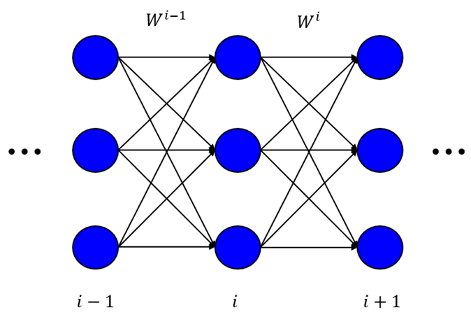
Note that the definition given above implies that ![]() refers to the weights from layer
refers to the weights from layer ![]() to layer
to layer ![]() , i.e. the weights 'going out of' layer
, i.e. the weights 'going out of' layer ![]() . Thus, the input layer has weights, but the output layer has no weights. I've illustrated this in the following figure.
. Thus, the input layer has weights, but the output layer has no weights. I've illustrated this in the following figure.
This is quite different from the conventions typically used today, e.g. in Keras. According to the conventions most widely used today, ![]() refers to the weights from layer
refers to the weights from layer ![]() to layer
to layer ![]() , i.e. the weights 'going into' layer
, i.e. the weights 'going into' layer ![]() . Thus, the output layer has weights, but the input layer has no weights. I've illustrated this in the following figure.
. Thus, the output layer has weights, but the input layer has no weights. I've illustrated this in the following figure.
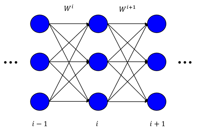
This is a fairly minor point, but is worth pointing out because it is an important detail to understand the subsequent derivation.
From these definitions we obtain the following:
![]()
(2)
![]()
(3)
Eqn. (2) is just the standard backpropagation formula for the partial derivatives of the cost function WRT the pre-activations, called the 'errors' or 'deltas' by some authors, usually written as ![]() (e.g. Bishop (2006)) - the things that get 'propagated backwards' through the network during network training. Eqn. (3) is then just the standard expression for the partials WRT the weights which can be used for gradient-based optimisation methods e.g. gradient descent.
(e.g. Bishop (2006)) - the things that get 'propagated backwards' through the network during network training. Eqn. (3) is then just the standard expression for the partials WRT the weights which can be used for gradient-based optimisation methods e.g. gradient descent.
The notation ![]() in (2) with the dot in the subscript in the original notation is a bit funny. All it means is we're taking the dot product of the vectors
in (2) with the dot in the subscript in the original notation is a bit funny. All it means is we're taking the dot product of the vectors ![]() and
and ![]() , as expected. For sake of clarity, I will rewrite Eqn. (2) as:
, as expected. For sake of clarity, I will rewrite Eqn. (2) as:
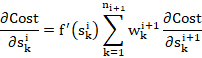
(2*)
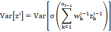
The variances will be expressed WRT the input, output and weight initialisation randomness. Consider the hypothesis that we are in a linear regime at the initialisation, that the weights are initialised independently and that the input feature variances are the same ![]() . Then we can say that, with
. Then we can say that, with ![]() the size of layer
the size of layer ![]() and
and ![]() the network input,
the network input,
![]()
(4)

(5)
We write ![]() for the shared scalar variance of all weights at layer
for the shared scalar variance of all weights at layer ![]() .
.
To derive Eqn. (5), consider the green unit in the network illustrated below.
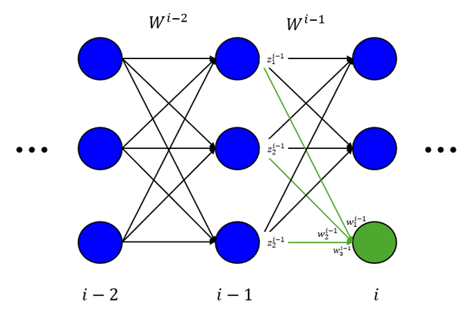
Using notation consistent with the paper, the forward propagation formula for the green unit is
Where ![]() is a sigmoidal activation function with the property that
is a sigmoidal activation function with the property that ![]() and where
and where ![]() indexes the units in layer
indexes the units in layer ![]() for the green unit specifically. Then
for the green unit specifically. Then
Because we assume we are in the linear regime of ![]() with approximately unit gradient (Eqn. (4)),
with approximately unit gradient (Eqn. (4)),
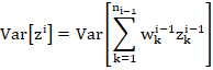
Because of the assumption of independence and zero-centredness of the weight and activation distributions,
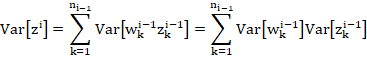
Because of the assumption of common activation variance for a given layer and common weight variance for a given layer,
![]()
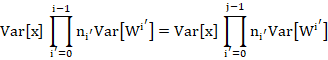
Thus we have a recursive expression for the variance of an activation as a function of the variance in the previous layer. Applying this recursively back to the input layer, and noting that ![]() ,
,
![]()

As claimed. QED.
Then for a network with ![]() layers,
layers,
(6)
(7)
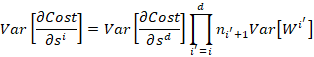
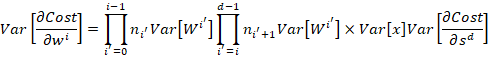
To derive Eqn. (6), we start with my expression for the backprop formula, Eqn. (2*), and take the variance of both sides:
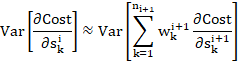
Where I have used the assumption that ![]() . Because of the assumption of independence and zero-centredness of the weight and error distributions,
. Because of the assumption of independence and zero-centredness of the weight and error distributions,
![]()
Similarly to the weights, we again have a recursive definition of the activation gradient variance for a layer as a function of the same thing in the next layer.
Using a line of reasoning identical to the analogous derivation for the activations, except starting from the output and working our way back recursively to the layer of interest instead of starting from the layer of interest and working our way back recursively to the input, gives Eqn. (6) as claimed.
Finally to get (7), just multiply (5) and (6). QED.
These two conditions transform to:
![]()
(10)
![]()
(11)
To derive (10), remember the AVC:
![]()
Consider two layers ![]() and
and ![]() . Substituting the expression for
. Substituting the expression for ![]() we derived (Eqn. (5)), the AVC says that:
we derived (Eqn. (5)), the AVC says that:
![]() and
and ![]() are arbitrary, so let
are arbitrary, so let ![]() . Then:
. Then:

Now, here is the key point: In order for this to hold for all ![]() , it must be the case that for all
, it must be the case that for all ![]() ,
,
![]()
Which is precisely Eqn. (10). An identical line of reasoning leads to the analogous expression Eqn. (11) for the EVC. QED.
As a compromise between these two constraints, we might want to have
![]()
(12)
Simply sum (10) and (11) and rearrange.
We call it the normalized initialisation:
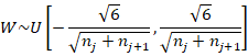
(16)
Finally, to go from (12) to (16), note that the variance of a continuous uniform distribution ![]() is given by
is given by ![]() . If the distribution is symmetric such that
. If the distribution is symmetric such that ![]() , its variance is
, its variance is ![]() . Equating this with (12),
. Equating this with (12),
![]()
Rearranging,
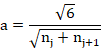
As claimed. QED. The completes the derivation of Glorot initialisation.
6 Conclusion
In this post, I have derived Glorot initialisation from first principles via a commentary on Glorot's paper, referring to his original derivation verbatim and filling in any details where more explanation could be provided for clarity.
7 References
Glorot, X. & Bengio, Y. 2010. Understanding the difficulty of training deep feedforward neural networks. Proceedings of the Thirteenth International Conference on Artificial Intelligence and Statistics. Proceedings of Machine Learning Research, 9, 249-256. http://proceedings.mlr.press/v9/glorot10a.html