A foreshadow of my data science career in my engineering undergrad: Kriging
2023-10-06
Gaussian process regression StatisticsContents
- 1 Spatial interpolation: An important problem in hydrocarbon exploration
- 2 Stating the problem formally
- 3 Kriging: Gaussian process regression for the geosciences
- 4 How the covariance is specified in geostatistics: Variograms
- 5 Worked example: Ordinary kriging
- 5.1 1D ordinary kriging
- 5.2 Aside: Sampling from the prior
- 5.3 Aside: Visualising the prior covariance matrix
- 5.4 Kriging estimate: The mean of the posterior GP
- 5.5 Visualising the posterior covariance matrix
- 6 Higher dimensions: 2D ordinary kriging
- 7 Alternative derivation of kriging: Best linear unbiased predictor
- 7.1 Preamble: Linear estimation
- 7.2 Desirable properties of a linear estimator
- 7.3 The unbiasedness criterion
- 7.4 The minimum variance criterion
- 7.5 Showing the derivations give equivalent results
- 8 Limitations of kriging
- 8.1 Endnote: Alternative to fitting a variogram: Estimating model parameters using MLE
- 9 References
1 Spatial interpolation: An important problem in hydrocarbon exploration
Petroleum engineers solve many problems during the process of developing a hydrocarbon asset. One of them is assisting the exploration team to understand the reservoir - the rock in the ground that contains the oil and/or gas.
To do this, they follow the same procedure that a data scientist (DS) (or experimental physicist, or econometrician, or any 21st century data-driven professional) follows, namely:
- Collect and prepare data
- Analyse the data
- Build a model
- Make inferences
The main things they want to know about the reservoir are:
- Its volume
 . This in turn is determined by its thickness
  and areal extent
- How much void space the rock contains per unit volume (the porosity,
 )
) - The fraction of that pore volume occupied by valuable fluids (oil or gas) and worthless fluids (water) (the fluid saturations,
 )
) - Permeability: How easily the fluids can flow through the rock (the permeability,
 )
)
One of the ways of collecting data in the petroleum industry is to drill a hole, take out a sample of rock from the bottom of the hole, and perform laboratory measurements on that sample. Because each hole can cost from hundreds of thousands to several millions of dollars to drill, all else being equal we would like to drill as few of them as possible.
Suppose we drill a few of holes and take measurements of one of the above quantities from the sample extracted from each hole. Suppose we then want to estimate the value for that quantity at some new location far away from any of the holes. This is the problem of spatial interpolation.
2 Stating the problem formally
- Regionalised variable: A variable distributed throughout space and/or time. What mathematicians would call a scalar field.
- Random variable: A variable located at a given position which takes on values that follow a given probability distribution.
- Random function: The set of random variables for a given regionalised variable distributed throughout space or time.
- Realisation: A particular value of a random variable or random function.
With the above terminology in place, we can now restate the problem formally as follows:
Suppose we drill ![]() holes located at
holes located at ![]() , and we take a measurement of one of the above regionalised variables
, and we take a measurement of one of the above regionalised variables ![]() in each hole, so that we have observed one realisation
in each hole, so that we have observed one realisation ![]() of each of
of each of ![]() random variables
random variables ![]() . Our goal is to estimate the true realisations
. Our goal is to estimate the true realisations ![]() of the random variables
of the random variables ![]() for a set of
for a set of ![]() new locations
new locations ![]() .
.
3 Kriging: Gaussian process regression for the geosciences
Kriging is the term used by the geostatistics community for historical reasons to refer to Gaussian process regression (GPR). In GPR, we model the regionalised variable to be predicted as a Gaussian process (GP), a type of stochastic process. The regression problem then becomes one of estimating the mean and variance of the GP for the test set.
GPR gives linear estimates in these sense that each target prediction can be shown to be a linear combination of the training targets. The variance between target values for different input features is modelled by a kernel function ![]() , which must be an inner product in feature space. As is possible to show, this is equivalent to saying the Gram matrix
, which must be an inner product in feature space. As is possible to show, this is equivalent to saying the Gram matrix ![]() whose elements are
whose elements are ![]() is positive definite. Unlike, say, linear regression, GPR is a nonparametric method and as such its complexity grows with the size of the training set.
is positive definite. Unlike, say, linear regression, GPR is a nonparametric method and as such its complexity grows with the size of the training set.
Before proceeding, let's first define some notation: Uppercase ![]() , uppercase
, uppercase ![]() and lowercase
and lowercase ![]() .
.
Let ![]() be the known values of the regionalised variable of interest at sampled locations
be the known values of the regionalised variable of interest at sampled locations ![]() . This is our training set. Our goal is to predict the function values
. This is our training set. Our goal is to predict the function values ![]() at
at ![]() unsampled locations
unsampled locations ![]() . This requires that we evaluate the conditional distribution
. This requires that we evaluate the conditional distribution ![]() .
.
Let ![]() . Now
. Now ![]() , where
, where ![]() is the covariance matrix related to the Gram matrix as follows:
is the covariance matrix related to the Gram matrix as follows: ![]() , where
, where ![]() is the variance (autocovariance at lag 0) and
is the variance (autocovariance at lag 0) and ![]() is the identity matrix. We can partition
is the identity matrix. We can partition ![]() as follows:
as follows:
![]()
Where ![]() and
and ![]() are the covariance matrices for sampled and unsampled locations. Using well-established results for partitioned covariances matrices of multivariate Gaussians, we see that the conditional distribution
are the covariance matrices for sampled and unsampled locations. Using well-established results for partitioned covariances matrices of multivariate Gaussians, we see that the conditional distribution ![]() is a Gaussian with mean and covariance given by:
is a Gaussian with mean and covariance given by:
![]()
![]()
(GPR equations)
The kriging estimate is simply this posterior mean ![]() , and the posterior covariance
, and the posterior covariance ![]() additionally gives us a measure of the uncertainty in our estimate.
additionally gives us a measure of the uncertainty in our estimate.
The above two equations are the key results that define GPR. (Later on, I will show that the above expression for the mean of the GPR is in fact a best linear unbiased estimator (BLUP) for ![]() ).
).
What remains to be seen is how we specify the kernel function ![]() and in turn specify all the
and in turn specify all the ![]() and
and ![]() matrices. One approach is to estimate it using maximum likelihood estimation (more on this later). An alternative approach is to infer it from the data. For this, we turn to a popular tool in geostatistics: The variogram.
matrices. One approach is to estimate it using maximum likelihood estimation (more on this later). An alternative approach is to infer it from the data. For this, we turn to a popular tool in geostatistics: The variogram.
4 How the covariance is specified in geostatistics: Variograms
In geostatistics, the kernel function (and hence the covariance) is expressed using the so-called variogram. The variogram ![]() is defined as the expected squared difference between the values at two points
is defined as the expected squared difference between the values at two points ![]() and
and ![]() :
:
![]()
It can be shown that under the stationarity assumptions this reduces to:
![]()
Where ![]() , so that
, so that ![]() is the Euclidean distance between
is the Euclidean distance between ![]() and
and ![]() . Thus the variogram is the expected squared difference of values of the regionalised variable in different locations as a function of their distance apart. Further application of the stationary assumptions and algebraic manipulation shows that this can be written as a function of
. Thus the variogram is the expected squared difference of values of the regionalised variable in different locations as a function of their distance apart. Further application of the stationary assumptions and algebraic manipulation shows that this can be written as a function of ![]() only, as follows:
only, as follows:
![]()
Where ![]() . The function
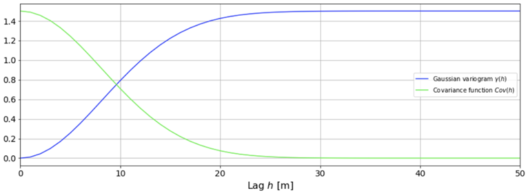
. The function ![]() equal to half the variogram is called the semivariogram. The semivariogram is often used instead of the variogram for convenience. I have illustrated the relationship between the semivariogram and autocovariance in the following figure.
equal to half the variogram is called the semivariogram. The semivariogram is often used instead of the variogram for convenience. I have illustrated the relationship between the semivariogram and autocovariance in the following figure.
To construct an empirical variogram, for every possible lag ![]() , we first find the subset
, we first find the subset ![]() and take its mean. (In practice, because we may have minimal data, we instead bin the data into subsets
and take its mean. (In practice, because we may have minimal data, we instead bin the data into subsets ![]() where
where ![]() is some small threshold). We then fit various semivariogram models to the data and select the one that has the best fit, perhaps drawing on experience in adjacent fields to use as analogs.
is some small threshold). We then fit various semivariogram models to the data and select the one that has the best fit, perhaps drawing on experience in adjacent fields to use as analogs.
The following figure illustrates a few popular variogram models. Range, sill and nugget are 20 m, 1 m2 and 0 m2, respectively.
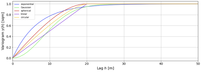
In particular, the Gaussian variogram is given by:
![]()
![]()
5 Worked example: Ordinary kriging
5.1 1D ordinary kriging
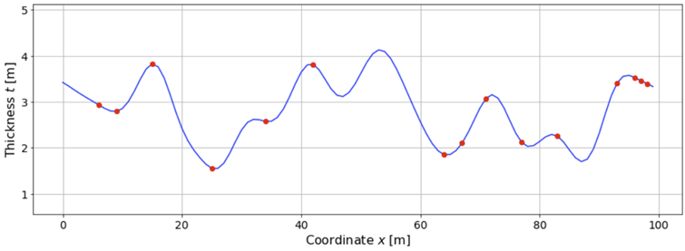
Suppose we are developing a reservoir. For simplicity, let's start with the assumption that most of its variation can be explained by a single direction, in which case we can model it as a 1D problem. Suppose we have drilled 10 holes and have taken laboratory measurements on rock samples extracted from those holes. The results are shown below.
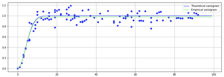
We then perform the aforementioned procedure to build the empirical variogram. The theoretical and empirical variogram are shown in the following figure.
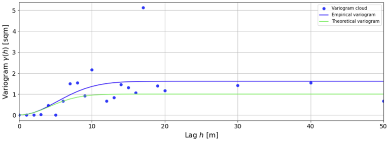
There is an entire body of literature on the best ways to fit empirical variograms. Here, for simplicity I have just used scipy.optimize with a squared-error objective function. Note that the empirical variogram grossly overestimates the true variogram. This reflects the fact that estimates of mean squared differences are biased. However, they are consistent, which means that in the limit of an infinite number of sampling experiments, the empirical variogram would perfectly reproduce the theoretical. To convince ourselves of this, and as a sense-check of our approach, we can perform a large number of sampling experiments and plot the variogram cloud. The results are shown in the following figure.
5.2 Aside: Sampling from the prior
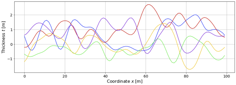
Suppose for sake of argument that before we drilled the holes, we had an idea of the variogram. Then we would have a prior distribution given by a GP with mean 0 and covariance matrix specified by the variogram:
![]()
The following figure shows a few sample functions drawn from this prior.
5.3 Aside: Visualising the prior covariance matrix
The following figure is a plot of the prior covariance matrix. It is a Toeplitz matrix, reflecting the fact that the prior GP is stationary.
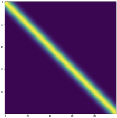
Later on, after we have drilled a few holes and performed laboratory measurements of core samples, we will compare this with the posterior covariance (N.B. this is not something done in practice but is useful for pedagogical purposes).
5.4 Kriging estimate: The mean of the posterior GP
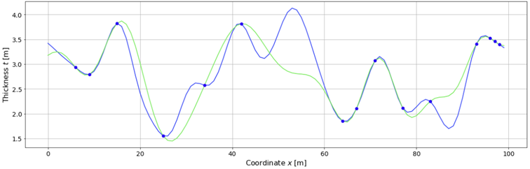
After we have drilled the holes and taken measurements, we update our prior belief (expressed by the prior GP) with data (AKA observations) to arrive at a posterior belief (our belief after-the-fact). The following figure shows samples drawn from this posterior.
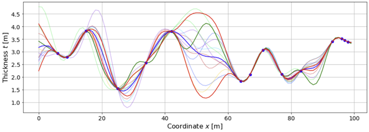
The kriging estimate is simply the expected value of this posterior GP. This is shown in the following figure. As we can see, it interpolates the true realisation reasonably well for densely sampled regions but less so for regions with few or no samples, particularly the region between Wells 6 and 7.
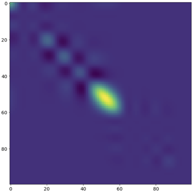
5.5 Visualising the posterior covariance matrix
The following figure is a visualisation of the posterior covariance matrix. It of course remains symmetric but is no longer Toeplitz, reflecting the fact that the posterior GP is nonstationary: The means are no longer identically zero but are equal the values at sampled locations, at which the variance is zero and covariance is higher for nearby unsampled points. The bright yellow patch represents the region of greatest uncertainty, between holes 6 and 7.
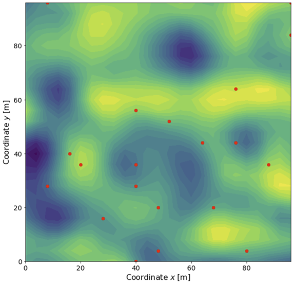
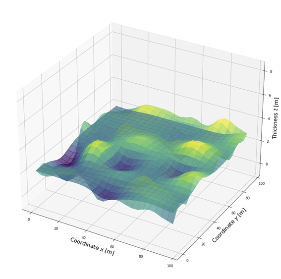
6 Higher dimensions: 2D ordinary kriging
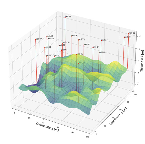
Suppose for geological reasons we could no longer make the 1D assumption and we had to model it in 2D. The above method applies to this 2D case (and any higher dimensions) with no modification. Suppose again we have drilled 10 holes and have taken laboratory measurements on rock samples extracted from those holes. The results are shown below.
2D view:
3D isometric view:
As before, we can estimate the surface using kriging:
2D slice at ![]() :
:
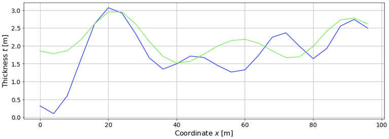
Note that in this case, we need to drill more holes and collect more data to accurately model the surface. In fact, the amount of data we need grows exponentially with the number of dimensions. This is a manifestation of the curse of dimensionality.
Now that I have defined kriging and provided worked examples, I think it is beneficial to discuss an alternative derivation of kriging which is more from a classic statistical perspective, compared to the derivation I presented first which is more from a modern machine learning (ML) perspective. The classic derivation I present in the following is in fact the one I learned first at university. Only later in my DS career I did I learn the ML derivation above, i.e. the derivation from the Gaussian process perspective. Crucially, the classic derivation reveals that kriging is the best linear unbiased predictor (BLUP) of the regionalised variable of interest.
7 Alternative derivation of kriging: Best linear unbiased predictor
7.1 Preamble: Linear estimation
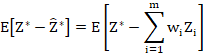
Suppose we wish to estimate the value for ![]() at an unsampled location using a linear estimate, i.e. by taking a linear combination of the values at each of the holes:
at an unsampled location using a linear estimate, i.e. by taking a linear combination of the values at each of the holes:

There are many ways we could come up with the weights ![]() . For example, we could let the weight for the closest data point be equal to 1 and the rest be equal to 0. This is the nearest neigbhour (NN) estimate.
. For example, we could let the weight for the closest data point be equal to 1 and the rest be equal to 0. This is the nearest neigbhour (NN) estimate.
Or as a generalisation of this, we could let the weights for the closest ![]() data points be equal to
data points be equal to ![]() and the rest equal to
and the rest equal to ![]() . This is the k-nearest neighbour (kNN) estimate.
. This is the k-nearest neighbour (kNN) estimate.
Or we could set the weights equal to the normalised reciprocals of the distances between the existing locations and the new location:

![]()
This is the inverse distance weighting (IDW) estimate.
7.2 Desirable properties of a linear estimator
Each of the above approaches, while simple, is somewhat unsatisfying. They leave much to be desired from a statistical standpoint. In particular:
- While strictly speaking they do account for the correlation between related data points (see Tobler's first law of geography), they do so at best in only a very crude way and certainly not a data-driven way.
- They do not give us an estimate of the prediction uncertainty.
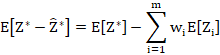
A question worth asking is: Given we want to make a linear estimate ![]() of
of ![]() , what are some requirements we want such an estimate to have? A statistician might answer this question as follows:
, what are some requirements we want such an estimate to have? A statistician might answer this question as follows:
- We want the estimate to be unbiased:
 . That is, we do not want our estimate to systemically over- or under-estimate the true value.
 - We want the estimate to be 'optimal' in some sense. A popular optimality criterion for an estimator is that it minimises the expected squared difference (or mean squared error, MSE) between the predicted value and the true values, over all possible realisations of the random function:
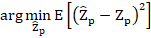 .
. - We want the estimate to honour known data:
 .
.
Under a set of assumptions, it is possible to show that kriging is the best linear unbiased predictor (BLUP) of the regionalised variable in question at unsampled locations.
What is a BLUP? It is a predictor with the following properties:
- Best: Among all possible unbiased linear predictors, it has the minimum variance.
- Linear: It is equal to a linear combination of the observations.
- Unbiased: Its expected value is equal to the true value.
7.3 The unbiasedness criterion
Before we proceed, a brief note on notation: For simplicity, because for the purpose of this derivation we are only considering a single point to be estimated, I will use the notation ![]() to refer to what I have called
to refer to what I have called ![]() previously. With this in mind, we have
previously. With this in mind, we have
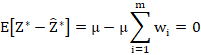

This shows that the requirement that it is unbiased implies that the kriging weights are normalised.
7.4 The minimum variance criterion
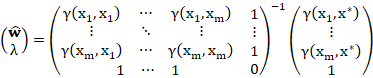
The coefficients ![]() can be determined from this equation and from condition (4), taking into account the constraint Eq. (7). This system of
can be determined from this equation and from condition (4), taking into account the constraint Eq. (7). This system of ![]() equations is solved by introducing (7) in (4) with a Lagrange multiplier
equations is solved by introducing (7) in (4) with a Lagrange multiplier ![]() . The Lagrange multiplier is an additional unknown constant which makes the number of unknown parameters equal to the number of equations.
. The Lagrange multiplier is an additional unknown constant which makes the number of unknown parameters equal to the number of equations.
The system of linear equations for which ![]() and
and ![]() must be solved is given by
must be solved is given by
The Lagrangian is
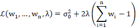
![]()
The partial derivatives of condition (8) yield (7) and a system of ![]() linear equations:
linear equations:
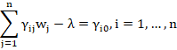

In matrix form:
7.5 Showing the derivations give equivalent results
Considering the system for ![]() only, taking the transpose of both sides and right-multiplying by
only, taking the transpose of both sides and right-multiplying by ![]() ,
,
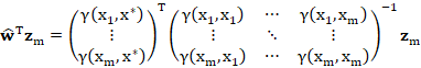
But the matrices on the RHS are just ![]() and
and ![]() defined previously! Substituting these,
defined previously! Substituting these,
![]()
Which is precisely the same as the posterior mean ![]() of the Gaussian process derived previously in the GPR equations! This shows that the mean of the GP is indeed a BLUP for
of the Gaussian process derived previously in the GPR equations! This shows that the mean of the GP is indeed a BLUP for ![]() . QED.
. QED.
8 Limitations of kriging
- As with any method, if the assumptions do not hold, kriging might not perform well.
- There might be better nonlinear and/or biased methods.
- No properties are guaranteed when the wrong variogram is used. However, typically still a 'good' interpolation is achieved.
- Best is not necessarily 'good': E.g. in the case of no spatial dependence the kriging interpolation is only as good as the arithmetic mean.
- Kriging provides
 as a measure of precision. However, this measure relies on the correctness of the variogram.
8.1 Endnote: Alternative to fitting a variogram: Estimating model parameters using MLE
Instead of specifying the covariance via an empirical variogram, we could have estimated it using maximum likelihood estimation (MLE). The log marginal likelihood is given by:
![]()
The partial derivatives are given by:
![]()
Details of an algorithm for a practical implementation of the above is beyond the scope of this post. In short, it involves performing a Cholesky decomposition of ![]() and solving two linear systems of equations involving the resulting lower triangular matrix. The interested reader should refer to Chapter 2 of Rasmussen (2006).
and solving two linear systems of equations involving the resulting lower triangular matrix. The interested reader should refer to Chapter 2 of Rasmussen (2006).
9 References
Bárdossy, A. Introduction to geostatistics.
Bay, X., Gauthier, B. 2010. Extended formula for kriging interpolation.
Bishop, C. M., 2006. Pattern recognition and machine learning.
Ginsbourger, D. et. al. 2008. A note on the choice and the estimation of kriging models for the analysis of deterministic computer experiments.
Le, N. D., Zidek, J. V., 1992. Interpolation with uncertain spatial covariances: A Bayesian alternative to kriging.
Malvic, T., Balic, D. 2010. Linearity and Lagrange linear multiplicator in the equations of ordinary kriging.
Mønness, E., Coleman, S. 2011. A short note on variograms and correlograms.
Rasmussen, C. E., Williams, K. I., 2005. Gaussian processes for machine learning.
Ro, Y., Yoo, C. 2022. Numerical experiments applying simple kriging to intermittent and log-normal data.
Sjöstedt-De Luna, S., Young, A., 2003. The bootstrap and kriging prediction intervals.
Wilson, J. T. et. al. 2020. Efficiently sampling functions from Gaussian process posteriors.